DNA metabarcoding diet analysis in reindeer is quantitative and integrates feeding over several weeks

Authors

Affiliations

Stefaniya Kamenova

Centre for Ecological and Evolutionary Synthesis, University of Oslo

Departments of Ecology and Natural Resource Management, Norwegian University of Life Sciences

National Museum of Natural History, Bulgarian Academy of Sciences

Pernille Meyer

Centre for Ecological and Evolutionary Synthesis, University of Oslo

Anne Krag Brysting

Centre for Ecological and Evolutionary Synthesis, University of Oslo

Leo Rescia

Department of Arctic and Marine Biology, The Arctic University of Norway

Lars P. Folkow

Department of Arctic and Marine Biology, The Arctic University of Norway

Galina Gusarova

Centre for Ecological and Evolutionary Synthesis, University of Oslo

Department of Arctic and Marine Biology, The Arctic University of Norway

The Arctic University Museum of Norway, The Arctic University of Norway

Department of Botany, St Petersburg State University

Eric Coissac

Laboratoire d’Ecologie Alpine, CNRS, Université Grenoble Alpes

Abstract

Filtering of the EUKA02 DNA metabarcoding raw data.

Setting up the R environment

Install missing packages

packages <- c(
  "tidyverse", "devtools", "vegan",
  "ggpubr", "colorspace", "R.utils", "ggthemes",
  "ggforce"
)

install.packages(
  setdiff(
    packages,
    rownames(installed.packages())
  ),
  dependencies = TRUE
)

Loads the used R packages

ROBITools package is used to read result files produced by OBITools.
ROBITaxonomy package provides function allowing to query OBITools formated taxonomy.

if (!"ROBITools" %in% rownames(installed.packages())) {
  # ROBITools are not available on CRAN and have to be installed
  # from http://git.metabarcoding.org using devtools

  metabarcoding_git <- "https://git.metabarcoding.org/obitools"

  devtools::install_git(paste(metabarcoding_git,
    "ROBIUtils.git",
    sep = "/"
  ))

  devtools::install_git(paste(metabarcoding_git,
    "ROBITaxonomy.git",
    sep = "/"
  ))
  devtools::install_git(paste(metabarcoding_git,
    "ROBITools.git",
    sep = "/"
  ))
}

library(ROBITools)
library(ROBITaxonomy)

tidyverse (Wickham et al., 2019) provides various methods for efficient data manipulation and plotting via ggplot2 (Wickham, 2016)

library(tidyverse)

vegan is loaded for its decostand function (Oksanen et al., 2015)

library(vegan)

ggthemes is loaded for its theme_tufte function

library(ggthemes)

ggpubr is loaded for its ggarrange function (Kassambara and Kassambara, 2020)

library(ggpubr)

library(colorspace)

library(R.utils)

library(magrittr)

Initialising some global data

The blind color compliant color pallet for plant families.

family_color <- c(
  "#991919", "#fcff5d",
  "#0ec434", "#228c68", "#8ad8e8", "#235b54", "#29bdab",
  "#3998f5", "#37294f", "#277da7", "#3750db", "#f22020",
  "#ffc413", "#f47a22", "#2f2aa0", "#b732cc", "#772b9d",
  "#5d4c86"
)

# The palette with grey:
cbPalette <- c("#999999", "#E69F00", "#56B4E9", 
               "#009E73", "#F0E442", "#0072B2", 
               "#D55E00", "#CC79A7")

# The palette with black:
cbbPalette <- c("#000000", "#E69F00", "#56B4E9", 
                "#009E73", "#F0E442", "#0072B2", 
                "#D55E00", "#CC79A7")

Reading the data

Reading of the NCBI taxonomy

taxo = read.taxonomy("Data/ncbi20210212")

Reading of the metabarcoding data

For the EUKA02 data set

The Read contingency table

reads <- read_csv("Data/Faeces/FE.Eukaryota.samples.reads.csv",
  show_col_types = FALSE
) %>%
  column_to_rownames("id") %>%
  as.matrix() %>%
  decostand(method = "total")

The sample description table

samples <- read_csv("Data/Faeces/FE.Eukaryota.samples.samples.csv",
  show_col_types = FALSE
) %>%
  mutate(.id = sample_id) %>%
  column_to_rownames(".id") %>%
  mutate(
    Animal_id = factor(Animal_id,
      levels = c("9/10", "10/10", "12/10")
    ),
    Fed_biomass = factor(Fed_biomass,
      levels = c("20", "500", "2000")
    )
  )

The MOTU description table

motus <- read_csv("Data/Faeces/FE.Eukaryota.samples.motus.csv",
  show_col_types = FALSE
) %>%
  mutate(.id = id) %>%
  column_to_rownames(".id")

Create a metabarcoding.data object, where you merge the three tables

Euka02 <- metabarcoding.data(
  reads = reads,
  samples = samples,
  motus = motus
)

And sorts the table from the most to the less abundante MOTU.

motus.hist <- colMeans(reads(Euka02))
Euka02@motus$mean_ref_freq <- motus.hist
Euka02 <- Euka02[, order(motus.hist, decreasing = TRUE)]

For the SPER01 data set

The Read contingency table

reads <- read_csv("Data/Faeces/FE.Spermatophyta.samples.reads.csv",
  show_col_types = FALSE
) %>%
  column_to_rownames("id") %>%
  as.matrix() %>%
  decostand(method = "total")

The sample description table

samples <- read_csv("Data/Faeces/FE.Spermatophyta.samples.samples.csv",
  show_col_types = FALSE
) %>%
  mutate(.id = sample_id) %>%
  column_to_rownames(".id") %>%
  mutate(
    Animal_id = factor(Animal_id,
      levels = c("9/10", "10/10", "12/10")
    ),
    Fed_biomass = factor(Fed_biomass,
      levels = c("20", "500", "2000")
    )
  )

The MOTU description table

motus <- read_csv("Data/Faeces/FE.Spermatophyta.samples.motus.csv",
  show_col_types = FALSE
) %>%
  mutate(.id = id) %>%
  column_to_rownames(".id")

Create a metabarcoding.data object, where you merge the three tables

Sper01 <- metabarcoding.data(
  reads = reads,
  samples = samples,
  motus = motus
)

And sorts the table from the most to the less abundante MOTU.

motus.hist <- colMeans(reads(Sper01))
Sper01@motus$mean_ref_freq <- motus.hist
Sper01 <- Sper01[, order(motus.hist, decreasing = TRUE)]

An overview of the diet

MOTUs are aggregated at family level.

Sper01_family <- aggregate(Sper01, by = list(family = Sper01@motus$family_name), MARGIN = 2, FUN = sum)

Euka02@motus %<>%
  mutate(family_name = ifelse(category == "Lichen",
    "Lecanoromycetidae",
    family_name
  ))
Euka02_family <- aggregate(Euka02,
  by = list(family = Euka02@motus$family_name),
  MARGIN = 2,
  FUN = sum
)

Sper01_family@reads %>%
  as.data.frame() %>%
  rownames_to_column("sample_id") %>%
  left_join(Sper01_family@samples,
    by = join_by(sample_id)
  ) %>%
  group_by(Animal_id) %>%
  summarise(across(
    where(is.numeric),
    ~ mean(.x, na.rm = TRUE)
  )) %>%
  select(Animal_id, ends_with("aceae")) %>%
  pivot_longer(-Animal_id,
    names_to = "Family",
    values_to = "RRA"
  ) -> diet_sper01

Euka02_family@reads %>%
  decostand(method = "total") %>%
  as.data.frame() %>%
  rownames_to_column("sample_id") %>%
  left_join(Euka02_family@samples,
    by = join_by(sample_id)
  ) %>%
  group_by(Animal_id) %>%
  summarise(across(
    where(is.numeric),
    ~ mean(.x, na.rm = TRUE)
  )) %>%
  select(Animal_id, ends_with("ae")) %>%
  pivot_longer(-Animal_id,
    names_to = "Family",
    values_to = "RRA"
  ) -> diet_euka02

diet_sper01 %>%
  mutate(Marker = "SPER01") %>%
  bind_rows(diet_euka02 %>% 
              mutate(Marker = "EUKA02")) %>%
  mutate(Marker = factor(Marker,
    levels = c("SPER01", "EUKA02")
  )) %>%
  group_by(Family) %>%
  mutate(
    merge = mean(RRA) < 0.01,
    Family = ifelse(merge, "Others", Family)
  ) %>%
  group_by(Family, Marker, Animal_id) %>%
  summarise(RRA = sum(RRA), .groups = "drop") -> diet_data

Families <- diet_data$Family %>%
  unique() %>%
  setdiff(c(
    "Lecanoromycetidae",
    "Betulaceae",
    "Others"
  )) %>%
  c(
    "Lecanoromycetidae",
    "Betulaceae",
    .,
    "Others"
  )

diet_data %>%
  mutate(Family = factor(Family, levels = Families)) %>%
  ggplot(aes(x = Animal_id, y = RRA, fill = Family)) +
  geom_col() +
  facet_wrap(. ~ Marker) +
  xlab("Animals") +
  ylab("Relative read abundances") +
  scale_fill_manual(
    name = "Families",
    values = family_color
  ) +
  theme(
    axis.title.x = ggtext::element_markdown(),
    axis.title.y = ggtext::element_markdown()
  ) -> comparative_diet_plot

ggsave("Figures/comparative_diet.pdf",
  comparative_diet_plot,
  dpi = 300,
  width = 20, height = 10, units = c("cm")
)
ggsave("Figures/comparative_diet.tiff",
  comparative_diet_plot,
  dpi = 300,
  width = 20, height = 10, units = c("cm")
)

comparative_diet_plot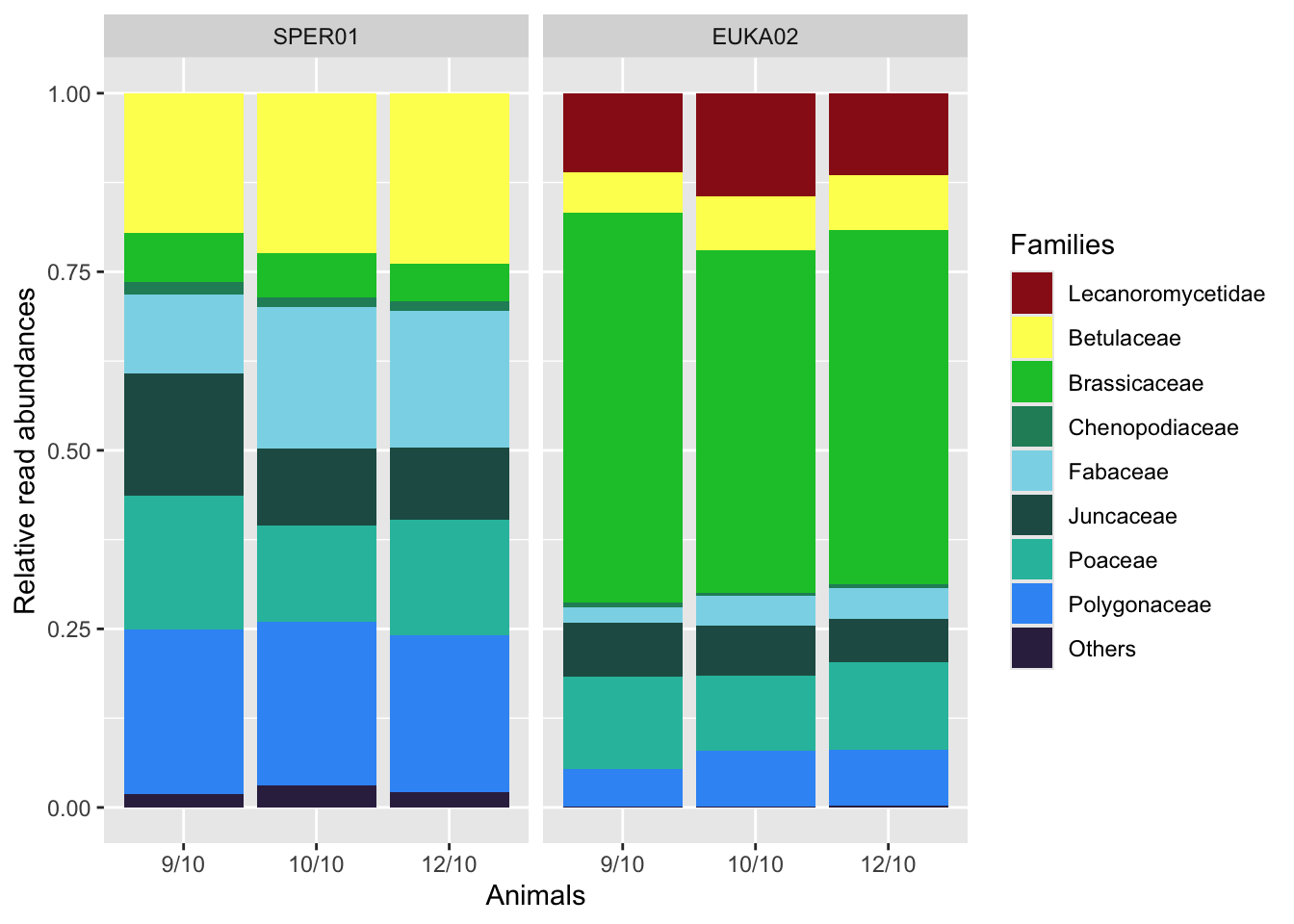

Families representing less than one percent of the average diet with both markers are collapsed into the ‘Others’ category. Lecanoromycetidae is actually a sub-class and corresponds to the MOTUs representing the lichens in the EUKA02 diet data.

diet_data %>%
  pivot_wider(names_from = c("Animal_id","Marker"),values_from = "RRA") %>%
  mutate(Family = factor(Family,levels = Families)) %>%
  arrange(Family) %>%
  mutate_if(is.numeric,~ round(.,3))

Analysis of the diet

Evolution of the Food items accross time

For the Euka02 marker

Euka02_family@reads %>% 
  as.data.frame() %>% 
  rownames_to_column("sample_id") %>%
  pivot_longer(cols = - "sample_id", names_to = "Family",values_to = "RRA") %>%
  mutate(Family = factor(Family,levels=Families)) %>%
  left_join(Euka02@samples, by = "sample_id")  %>%
  mutate(times_from_birch = times_from_birch/24) %>%
  filter(! is.na(Family)) %>%
  filter(! is.na(RRA)) %>%
  filter(times_from_birch >=-2 & times_from_birch <= 25 ) %>%
  ggplot(aes(x=times_from_birch,y=RRA, col = Animal_id)) +
  geom_point(size=0.5) +
  xlim(-2,25) + 
  facet_wrap(. ~ Family, ncol=2,scales="free_y") +
  geom_vline (xintercept = 0.54, colour = "lightgrey") +
  geom_vline (xintercept = 1.54, colour = "lightgrey") +
  geom_vline (xintercept = 2.54, colour = "lightgrey") +
  geom_vline (xintercept = 5.54, colour = "lightgrey") + 
  geom_vline (xintercept = 6.54, colour = "lightgrey") + 
  geom_vline (xintercept = 7.54, colour = "lightgrey") + 
  geom_vline (xintercept = 10.54, colour = "lightgrey") +
  geom_vline (xintercept = 11.54, colour = "lightgrey") +
  geom_vline (xintercept = 12.54, colour = "lightgrey") +
  annotate("text", x = 1.60, y = 1, label = "20g",size = 3) + 
  annotate("text", x = 6.60, y = 1, label = "500g",size = 3) +
  annotate("text", x = 11.60, y = 1, label = "2000g",size = 3) +
  ylab("Relative reads abundance") +
  xlab("Time (days after *Betula pubescens* was fed)") +
  theme_bw() +
  theme(axis.title.x = ggtext::element_markdown(),
        legend.position="bottom") + 
  scale_color_manual(name="Animal",values = family_color) -> euka02_family_plot

ggsave("Figures/Euka02_family_plot.pdf",
       euka02_family_plot,
       dpi = 300,
      width = 32, height = 35, units = c("cm"))

ggsave("Figures/Euka02_family_plot.tiff",
       euka02_family_plot,
       dpi = 300,
      width = 16, height = 17, units = c("cm"))

euka02_family_plot

For the Sper01 marker

Sper01_family@reads %>% 
  as.data.frame() %>% 
  rownames_to_column("sample_id") %>%
  pivot_longer(cols = - "sample_id", names_to = "Family",values_to = "RRA") %>%
  mutate(Family = factor(Family,levels=Families)) %>%
  left_join(Sper01@samples, by = "sample_id")  %>%
  mutate(times_from_birch = times_from_birch/24) %>%
  filter(! is.na(Family)) %>%
  filter(! is.na(RRA)) %>%
  filter(times_from_birch >=-2 & times_from_birch <= 25 ) %>%
  ggplot(aes(x=times_from_birch,y=RRA, col = Animal_id)) +
  geom_point(size=0.5) +
  xlim(-2,25) + 
  facet_wrap(. ~ Family, ncol=2,scales="free_y") +
  geom_vline (xintercept = 0.54, colour = "lightgrey") +
  geom_vline (xintercept = 1.54, colour = "lightgrey") +
  geom_vline (xintercept = 2.54, colour = "lightgrey") +
  geom_vline (xintercept = 5.54, colour = "lightgrey") + 
  geom_vline (xintercept = 6.54, colour = "lightgrey") + 
  geom_vline (xintercept = 7.54, colour = "lightgrey") + 
  geom_vline (xintercept = 10.54, colour = "lightgrey") +
  geom_vline (xintercept = 11.54, colour = "lightgrey") +
  geom_vline (xintercept = 12.54, colour = "lightgrey") +
  annotate("text", x = 1.60, y = 1, label = "20g",size = 3) + 
  annotate("text", x = 6.60, y = 1, label = "500g",size = 3) +
  annotate("text", x = 11.60, y = 1, label = "2000g",size = 3) +
  ylab("Relative reads abundance") +
  xlab("Time (days after *Betula pubescens* was fed)") +
  theme_bw() +
  theme(axis.title.x = ggtext::element_markdown(),
        legend.position="bottom") + 
  scale_color_manual(name="Animal",values = family_color)  -> sper01_family_plot

ggsave("Figures/Sper01_family_plot.pdf",
       sper01_family_plot,
       dpi = 300,
      width = 32, height = 35, units = c("cm"))

ggsave("Figures/Sper01_family_plot.tiff",
       sper01_family_plot,
       dpi = 300,
      width = 16, height = 17, units = c("cm"))

sper01_family_plot

Normalisation of the Diet by a constant item

In the relative read frequency approach, the sum of all elements is, by definition, equal to one. This means that one degree of freedom is lost. Thus, if one item increases (birch or lichen in our experience), other items are forced to decrease because of the lost degree of freedom. Throughout the experiment, pellets were provided in a constant amount and therefore must be constantly retrieved in the feces. To recover the degree of freedom, the relative frequencies of the food items are divided by the pellet components. The new amount of food is therefore expressed in an arbitrary unit of DNA, and the amounts don’t add up to one in every sample.

Normalizing the `Euka02` data set

Euka02_family@motus %<>% 
  mutate(food = ifelse(family_name =="Betulaceae","Birch",
                       ifelse(family_name =="Lecanoromycetidae","Lichen","Pellet")))

Euka02_food <- aggregate(Euka02_family,MARGIN = "motus",
                         by=list(Food=Euka02_family@motus$food),
                         FUN = sum)


Euka02_food$dna_amount <- sweep(Euka02_food@reads,
                                  MARGIN = 1,
                                  STATS = Euka02_food@reads[,"Pellet"],
                                  FUN = "/"
                                 ) %>%
                          sweep(MARGIN = 1,
                                  STATS = Euka02_food@samples$pellets,
                                  FUN = "*"
                                 )

Normalizing the `Sper01` data set

Sper01_family@motus %<>% 
  mutate(food = ifelse(family_name =="Betulaceae","Birch",
                       ifelse(family_name =="Lecanoromycetidae","Lichen","Pellet")))

Sper01_food <- aggregate(Sper01_family,MARGIN = "motus",
                         by=list(Food=Sper01_family@motus$food),
                         FUN = sum)

Sper01_food$dna_amount <- sweep(Sper01_food@reads,
                                  MARGIN = 1,
                                  STATS = Sper01_food@reads[,"Pellet"],
                                  FUN = "/"
                                 ) %>%
                          sweep(MARGIN = 1,
                                  STATS = Sper01_food@samples$pellets,
                                  FUN = "*"
                                 )

Euka02_food$dna_amount %>%
  as.data.frame() %>%
  rownames_to_column("sample_id") %>%
  pivot_longer(cols = - "sample_id", names_to = "Food",values_to = "amount") %>%
  left_join(Euka02_food@samples, by = "sample_id") %>%
  mutate(times_from_birch = times_from_birch/24,
         time_group = floor(times_from_birch)) %>% 
  filter(Food=="Lichen") %>%
  filter(amount > 0) %>%
  filter(times_from_birch <= 26) -> lichen_data_Euka02

lichen_start_time=13
lichen_end_time=24

ggplot(data = lichen_data_Euka02, 
                      aes(x = times_from_birch,
                          y =  amount,
                          color = Animal_id)) +
  geom_point() + 
  geom_smooth(data = lichen_data_Euka02 %>% 
                filter(times_from_birch >= lichen_start_time & 
                       times_from_birch <= lichen_end_time),
              method = MASS::rlm,show.legend = FALSE,
              formula = y~x) + 
  scale_color_manual(values=cbbPalette) +
  stat_summary_bin(fun = median, geom = "line") +
  scale_y_log10() + 
  geom_vline (xintercept = c(0.54,1.54,2.54), colour = cbbPalette[6]) +
  geom_vline (xintercept = c(5.54,6.54,7.54), colour = cbbPalette[7]) + 
  geom_vline (xintercept = c(10.54,11.54,12.54), colour = cbbPalette[8]) +
  scale_x_continuous(breaks = scales::pretty_breaks(n = 15),limits = c(-2,25)) +
  guides(color=guide_legend(title="Individual")) +
  theme_minimal() +
  theme(panel.grid.major = element_blank(),
        panel.grid.minor = element_blank(),
        panel.background = element_blank(), 
        axis.title.x = ggtext::element_markdown(),
        axis.title.y = ggtext::element_markdown(), 
        axis.line = element_line(colour = "black")) +
  ylab("Amount of *Lecanoromycetidae* DNA") +
  xlab('Time (days after *Betula pubescens* was fed) in days') -> decay_leuca_euka02

decay_leuca_euka02

Warning in rlm.default(x, y, weights, method = method, wt.method = wt.method, :
'rlm' failed to converge in 20 steps

Euka02_food$dna_amount %>%
  as.data.frame() %>%
  rownames_to_column("sample_id") %>%
  pivot_longer(cols = - "sample_id", names_to = "Food",values_to = "amount") %>%
  left_join(Euka02_food@samples, by = "sample_id") %>%
  mutate(times_from_birch = times_from_birch/24,
         time_group = floor(times_from_birch)) %>% 
  filter(Food=="Birch") %>%
  filter(amount > 0) %>%
  filter(times_from_birch <= 25) -> birch_data_Euka02

birch_start_time=1
birch_end_time=10

ggplot(data = birch_data_Euka02, 
                      aes(x = times_from_birch,
                          y =  amount,
                          color = Animal_id)) +
  geom_point(size=1) + 
  geom_smooth(data = birch_data_Euka02 %>% 
                filter(times_from_birch >= birch_start_time & 
                       times_from_birch <= birch_end_time),
              method = MASS::rlm,
              show.legend = FALSE,
              formula = y~x) + 
  scale_color_manual(values=cbbPalette) +
  stat_summary_bin(fun = median, geom = "line") +
  scale_y_log10() + 
  geom_vline (xintercept = c(0.54,1.54,2.54), colour = cbbPalette[6]) +
  geom_vline (xintercept = c(5.54,6.54,7.54), colour = cbbPalette[7]) + 
  geom_vline (xintercept = c(10.54,11.54,12.54), colour = cbbPalette[8]) +
  scale_x_continuous(breaks = scales::pretty_breaks(n = 15),
                     limits = c(-2,25)) +
  guides(color=guide_legend(title="Individual")) +
  theme_minimal() +
  theme(panel.grid.major = element_blank(),
        panel.grid.minor = element_blank(),
        panel.background = element_blank(), 
        axis.title.x = ggtext::element_markdown(),
        axis.title.y = ggtext::element_markdown(),
        axis.line = element_line(colour = "black")) +
  ylab("Amount of *Betulaceae* DNA") +
  xlab('Time (days after *Betula pubescens* was fed) in days') -> decay_betula_euka02

decay_betula_euka02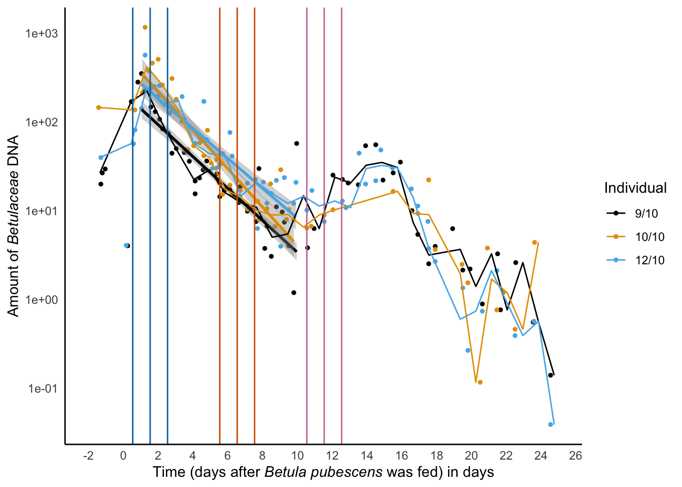

ggarrange(decay_betula_euka02,
          decay_leuca_euka02,
          common.legend = TRUE,
          legend="right",labels = c("A","B")) -> decay_euka02_plot

Warning in rlm.default(x, y, weights, method = method, wt.method = wt.method, :
'rlm' failed to converge in 20 steps

ggsave("Figures/decay_euka02.pdf",
       decay_euka02_plot,
       dpi=300,
       width=12,height=5)
ggsave("Figures/decay_euka02.tiff",
       decay_euka02_plot,
       dpi=300,
       width=12,height=5)
decay_euka02_plot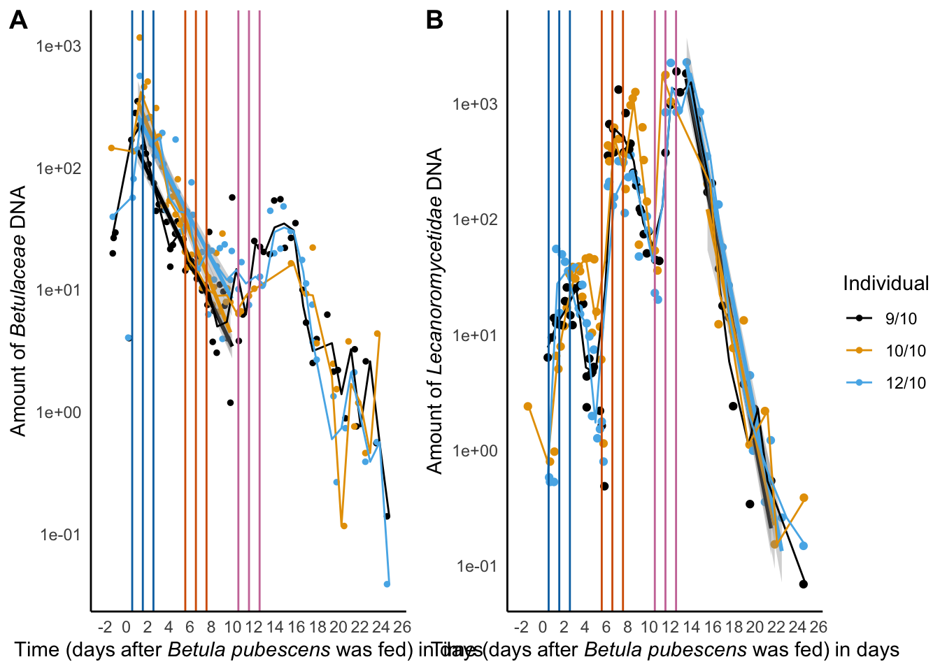

Estimate of the Half-time detection

lichen_data_Euka02 %>%
  filter(times_from_birch >= lichen_start_time &
    times_from_birch <= lichen_end_time) %>%
  MASS::rlm(times_from_birch ~ log(amount):Animal_id + Animal_id,
    data = .
  ) %>%
  summary() %>%
  .[["coefficients"]] %>%
  as.data.frame() %>%
  rownames_to_column("Effect") %>%
  filter(str_starts(Effect, "log")) %>%
  mutate(Animal = str_replace(Effect, "^.*Animal_id", "")) %>%
  bind_rows(
    lichen_data_Euka02 %>%
      filter(times_from_birch >= lichen_start_time &
        times_from_birch <= lichen_end_time) %>%
      MASS::rlm(times_from_birch ~ log(amount) + Animal_id, data = .) %>%
      summary() %>% .[["coefficients"]] %>%
      as.data.frame() %>%
      rownames_to_column("Effect") %>%
      filter(Effect == "log(amount)") %>%
      mutate(Animal = "All")
  ) %>%
  mutate(
    HalfTime = -Value * log(2) * 24,
    HalfTime_sd = `Std. Error` * log(2) * 24,
    HalfTime_ci_low = qnorm(0.025, mean = HalfTime, sd = HalfTime_sd),
    HalfTime_ci_high = qnorm(0.975, mean = HalfTime, sd = HalfTime_sd)
  ) %>%
  select(Animal, HalfTime, HalfTime_ci_low, HalfTime_ci_high, HalfTime_sd)

lichen_data_Euka02 %>%
      filter(times_from_birch >= lichen_start_time &
        times_from_birch <= lichen_end_time) %>%
      MASS::rlm(times_from_birch ~ log(amount) + Animal_id, data = .) %>%
      anova() %>% .["Sum Sq"] -> sq
sq/sum(sq)

birch_data_Euka02 %>%
  filter(times_from_birch >= birch_start_time &
    times_from_birch <= birch_end_time) %>%
  MASS::rlm(times_from_birch ~ log(amount):Animal_id + Animal_id,
    data = .
  ) %>%
  summary() %>%
  .[["coefficients"]] %>%
  as.data.frame() %>%
  rownames_to_column("Effect") %>%
  filter(str_starts(Effect, "log")) %>%
  mutate(Animal = str_replace(Effect, "^.*Animal_id", "")) %>%
  bind_rows(
    birch_data_Euka02 %>%
      filter(times_from_birch >= birch_start_time &
        times_from_birch <= birch_end_time) %>%
      MASS::rlm(times_from_birch ~ log(amount) + Animal_id, data = .) %>%
      summary() %>% .[["coefficients"]] %>%
      as.data.frame() %>%
      rownames_to_column("Effect") %>%
      filter(Effect == "log(amount)") %>%
      mutate(Animal = "All")
  ) %>%
  mutate(
    HalfTime = -Value * log(2) * 24,
    HalfTime_sd = `Std. Error` * log(2) * 24,
    HalfTime_ci_low = qnorm(0.025, mean = HalfTime, sd = HalfTime_sd),
    HalfTime_ci_high = qnorm(0.975, mean = HalfTime, sd = HalfTime_sd)
  ) %>%
  select(Animal, HalfTime, HalfTime_ci_low, HalfTime_ci_high, HalfTime_sd)

birch_data_Euka02 %>%
      filter(times_from_birch >= lichen_start_time &
        times_from_birch <= lichen_end_time) %>%
      MASS::rlm(times_from_birch ~ log(amount) + Animal_id, data = .) %>%
      anova() %>% .["Sum Sq"] -> sq
sq/sum(sq)

Sper01_food$dna_amount %>%
  as.data.frame() %>%
  rownames_to_column("sample_id") %>%
  pivot_longer(cols = - "sample_id", names_to = "Food",values_to = "amount") %>%
  left_join(Sper01_food@samples, by = "sample_id") %>%
  mutate(times_from_birch = times_from_birch/24,
         time_group = floor(times_from_birch)) %>% 
  filter(Food=="Birch") %>%
  filter(amount > 0) %>%
  filter(times_from_birch <= 25) -> birch_data_Sper01

birch_start_time=1
birch_end_time=10

ggplot(data = birch_data_Sper01, 
                      aes(x = times_from_birch,
                          y =  amount,
                          color = Animal_id)) +
  geom_point(size=1) + 
  geom_smooth(data = birch_data_Sper01 %>% 
                filter(times_from_birch >= birch_start_time & 
                       times_from_birch <= birch_end_time),
              method = MASS::rlm,
              show.legend = FALSE,
              formula = y~x) + 
  scale_color_manual(values=cbbPalette) +
  stat_summary_bin(fun = median, geom = "line") +
  scale_y_log10() + 
  geom_vline (xintercept = c(0.54,1.54,2.54), colour = cbbPalette[6]) +
  geom_vline (xintercept = c(5.54,6.54,7.54), colour = cbbPalette[7]) + 
  geom_vline (xintercept = c(10.54,11.54,12.54), colour = cbbPalette[8]) +
  scale_x_continuous(breaks = scales::pretty_breaks(n = 15),
                     limits = c(-2,25)) +
  guides(color=guide_legend(title="Individual")) +
  theme_minimal() +
  theme(panel.grid.major = element_blank(),
        panel.grid.minor = element_blank(),
        panel.background = element_blank(), 
        axis.title.x = ggtext::element_markdown(),
        axis.title.y = ggtext::element_markdown(),
        axis.line = element_line(colour = "black")) +
  ylab("Amount of *Betulaceae* DNA") +
  xlab('Time (days after *Betula pubescens* was fed) in days') -> decay_betula_sper01

decay_betula_sper01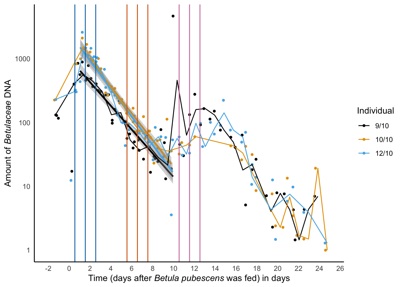

ggarrange(decay_betula_euka02,
          decay_betula_sper01,
          common.legend = TRUE,
          legend="right",labels = c("A","B")) -> decay_betula_plot
ggsave("Figures/decay_betula.pdf",
       decay_betula_plot,
       dpi=300,
       width=12,height=5)
ggsave("Figures/decay_betula.tiff",
       decay_betula_plot,
       dpi=300,
       width=12,height=5)
decay_betula_plot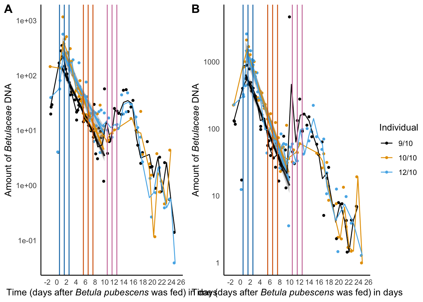

birch_data_Sper01 %>%
  filter(times_from_birch >= birch_start_time &
    times_from_birch <= birch_end_time) %>%
  MASS::rlm(times_from_birch ~ log(amount):Animal_id + Animal_id,
    data = .
  ) %>%
  summary() %>%
  .[["coefficients"]] %>%
  as.data.frame() %>%
  rownames_to_column("Effect") %>%
  filter(str_starts(Effect, "log")) %>%
  mutate(Animal = str_replace(Effect, "^.*Animal_id", "")) %>%
  bind_rows(
    birch_data_Sper01 %>%
      filter(times_from_birch >= birch_start_time &
        times_from_birch <= birch_end_time) %>%
      MASS::rlm(times_from_birch ~ log(amount) + Animal_id, data = .) %>%
      summary() %>% .[["coefficients"]] %>%
      as.data.frame() %>%
      rownames_to_column("Effect") %>%
      filter(Effect == "log(amount)") %>%
      mutate(Animal = "All")
  ) %>%
  mutate(
    HalfTime = -Value * log(2) * 24,
    HalfTime_sd = `Std. Error` * log(2) * 24,
    HalfTime_ci_low = qnorm(0.025, mean = HalfTime, sd = HalfTime_sd),
    HalfTime_ci_high = qnorm(0.975, mean = HalfTime, sd = HalfTime_sd)
  ) %>%
  select(Animal, HalfTime, HalfTime_ci_low, HalfTime_ci_high, HalfTime_sd)

birch_data_Sper01 %>%
      filter(times_from_birch >= lichen_start_time &
        times_from_birch <= lichen_end_time) %>%
      MASS::rlm(times_from_birch ~ log(amount) + Animal_id, data = .) %>%
      anova() %>% .["Sum Sq"] -> sq
sq/sum(sq)

ggplot(data = lichen_data_Euka02, 
                      aes(x = times_from_birch,
                          y =  amount,
                          color = Animal_id)) +
  geom_point() + 
  scale_color_manual(values=cbbPalette) +
  stat_summary_bin(fun = median, geom = "line") +
  scale_y_log10() + 
  geom_vline (xintercept = c(1.5,3.5), colour = cbbPalette[6]) +
  geom_vline (xintercept = c(6.5,8.5), colour = cbbPalette[7]) + 
  geom_vline (xintercept = c(11.5,13.5), colour = cbbPalette[8]) +
  scale_x_continuous(breaks = scales::pretty_breaks(n = 15),limits = c(-2,25)) +
  guides(color=guide_legend(title="Individual")) +
  theme_minimal() +
  theme(panel.grid.major = element_blank(),
        panel.grid.minor = element_blank(),
        panel.background = element_blank(), 
        axis.title.x = ggtext::element_markdown(),
        axis.title.y = ggtext::element_markdown(), 
        axis.line = element_line(colour = "black")) +
  ylab("Amount of *Lecanoromycetidae* DNA") +
  xlab('Time (days after *Betula pubescens* was fed) in days') -> decay_leuca_euka02

decay_leuca_euka02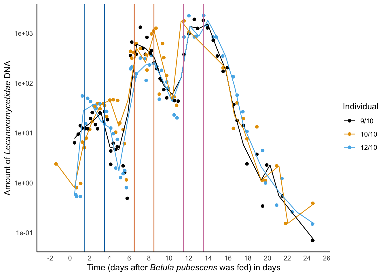

Euka02_food$dna_amount %>%
  as.data.frame() %>%
  rownames_to_column("sample_id") %>%
  pivot_longer(cols = -sample_id,names_to = "Food", values_to = "amount") %>%
  left_join(Euka02_food@samples, by = "sample_id") %>%
  mutate(maxi = ifelse(between(times_from_birch,1.5*24,3.5*24) | 
                        between(times_from_birch,6.5*24,8.5*24)| 
                        between(times_from_birch,11.5*24,13.5*24),"MAX","out")) %>%
  filter(!is.na(Fed_biomass)) %>%
  group_by(Animal_id,Fed_biomass,Food,maxi) %>%
  summarise(amount = median(amount),.groups = "drop") %>%
  filter(maxi == "MAX" & Food == "Lichen") %>%
  mutate(Fed_biomass = as.integer(as.character(Fed_biomass))) %>% 
  group_by(Animal_id) %>%
  mutate(amount = amount/sum(amount)*2520) -> food_dna_relation

  food_dna_relation %>%
    pivot_wider(names_from = Animal_id,values_from = amount)

food_dna_relation %>%
  ggplot(aes(x=Fed_biomass,y=amount)) +
  geom_point(aes(col=Animal_id)) +
  stat_smooth(method = lm,formula = 'y ~ x')+
  theme_classic() +  
  guides(color=guide_legend(title="Individual")) +
  scale_color_manual(values=cbbPalette) +
  labs(y="Amount of Lecanoromycetidae DNA") +
  labs(x=expression('Biomass of ingested lichen (g)'),
       fill="Var1")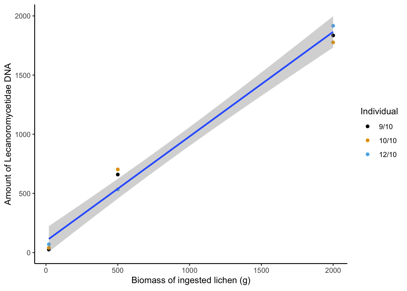

food_dna_relation %>%
  lm(amount ~ Fed_biomass + 1, data=.) -> dna_rra_lm

  summary(dna_rra_lm)


Call:
lm(formula = amount ~ Fed_biomass + 1, data = .)

Residuals:
   Min     1Q Median     3Q    Max 
-90.14 -74.76 -30.00  51.46 163.40 

Coefficients:
            Estimate Std. Error t value Pr(>|t|)    
(Intercept) 97.57730   46.48027   2.099   0.0739 .  
Fed_biomass  0.88384    0.03905  22.634 8.32e-08 ***
---
Signif. codes:  0 '***' 0.001 '**' 0.01 '*' 0.05 '.' 0.1 ' ' 1

Residual standard error: 98.79 on 7 degrees of freedom
Multiple R-squared:  0.9865,    Adjusted R-squared:  0.9846 
F-statistic: 512.3 on 1 and 7 DF,  p-value: 8.32e-08

  shapiro.test(residuals(dna_rra_lm))


    Shapiro-Wilk normality test

data:  residuals(dna_rra_lm)
W = 0.88313, p-value = 0.1694

References

Kassambara, A., Kassambara, M.A., 2020. Package “ggpubr.”

Oksanen, J., Blanchet, F.G., Kindt, R., Legendre, P., Minchin, P., O’Hara, R., Simpson, G., Solymos, P., Henry, M., Stevens, M., others, 2015. Vegan: Community ecology package. Ordination methods, diversity analysis and other functions for community and vegetation ecologists. R package ver 2–3.

Wickham, H., 2016. ggplot2: Elegant Graphics for Data Analysis. Springer-Verlag New York.

Wickham, H., Averick, M., Bryan, J., Chang, W., McGowan, L., François, R., Grolemund, G., Hayes, A., Henry, L., Hester, J., Kuhn, M., Pedersen, T., Miller, E., Bache, S., Müller, K., Ooms, J., Robinson, D., Seidel, D., Spinu, V., Takahashi, K., Vaughan, D., Wilke, C., Woo, K., Yutani, H., 2019. Welcome to the tidyverse. Journal of open source software 4, 1686. https://doi.org/10.21105/joss.01686

Other Formats

Setting up the R environment

Install missing packages

Loads the used R packages

Initialising some global data

Reading the data

Reading of the NCBI taxonomy

Reading of the metabarcoding data

For the EUKA02 data set

For the SPER01 data set

An overview of the diet

Analysis of the diet

Evolution of the Food items accross time

For the Euka02 marker

For the Sper01 marker

Normalisation of the Diet by a constant item

Normalizing the Euka02 data set

Normalizing the Sper01 data set

Estimate of the Half-time detection

References

Normalizing the `Euka02` data set

Normalizing the `Sper01` data set